CTI ECT Simulation

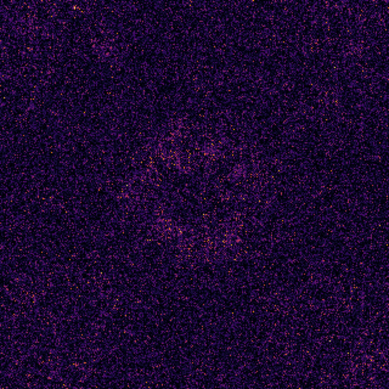
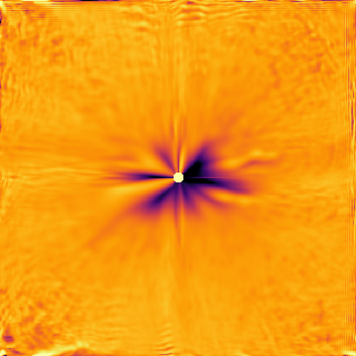
Raw density frame at late Stage-1, showing a stabilized compression halo.

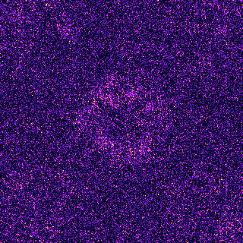
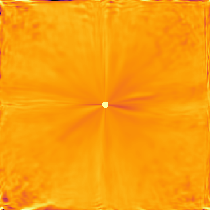
Same frame with contrast enhancement only. Geometry is unchanged.

Stage-1 serves as the numerical foundation for all subsequent ECT simulations. It demonstrates that the Primordial Wave Equation, equipped with a real compression functional, naturally generates a persistent halo structure from minimal symmetry-broken initial data. All later singularity, baryonic, and galaxy-scale simulations build directly on this stabilized compression geometry.

Collapse Sequence and Singularity Formation

The Stage-6 collapse shows that the same compression dynamics that stabilize halos also drive a sharply localized compression singularity once the energy density exceeds the stability threshold. The frames below show the emergence of the singularity directly from the Primordial Wave Equation with the ECT compression term, with no external potentials, no forcing, and no stochastic terms.

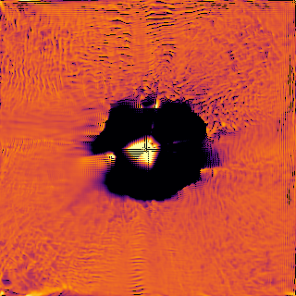
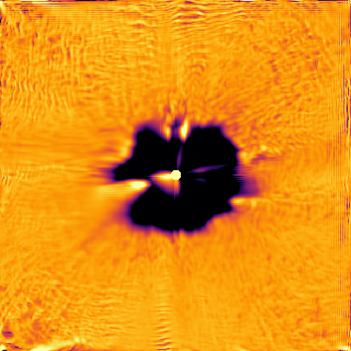
Four-frame Stage-6 collapse sequence. From left to right: birth of the mathematical singularity, early inner-halo collapse, late inward collapse (where baryons would accumulate along the boundary if present), and the final stabilized compression structure.

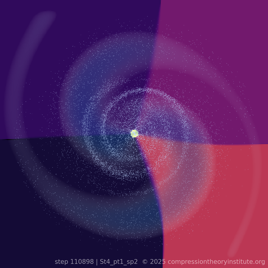
Continuation: Singularity to Galaxy Formation

The stabilized halo and compression singularity above serve as the substrate for the next phase. In the following simulation, baryonic matter and hydrogen are introduced as late-time asymmetric flows, producing sustained spiral structure within the same Primordial Wave Equation framework.

Download and run

You can download the complete Stage-1 simulation package as a single ZIP file, which includes the Python script, README.txt, all PNG frames, the MP4 video, the psi_final field, and the optional MP4 builder script.

• Download Stage-1 dataset (ECT_PWE_SIM_Stage1.zip)

Running the Stage-1 simulation

1. Install Python: Python 3.9 or later is recommended.
2. Install required packages:

   pip install numpy matplotlib

3. Place the script ECT_Dark_Halo_Stage1.py in an empty working directory and open a terminal in that directory.
4. Run the simulation:

   python ECT_Dark_Halo_Stage1.py

5. Outputs created in the local directory:
   • ECT_Dark_Halo_Stage_1_XXX.png (density snapshots at selected steps)
   • ECT_Dark_Halo_Stage_1_psi_final.npy (final complex wavefunction ψ)

Any modern desktop or laptop can run Stage-1. Typical runtime is on the order of 20 to 40 seconds on a recent 4-core CPU, depending on Python and NumPy builds.

How Stage-1 tests the PWE

The Primordial Wave Equation used in ECT is not a generic numerics toy. It is a specific deterministic equation that couples a Schrödinger like kinetic term to a real compression functional of the amplitude. The Stage-1 script provides a direct test of this equation in two dimensions with periodic boundary conditions and a physically motivated initial condition.

The halo that forms is not hand drawn or imposed. It is the result of:

• a single PWE with fixed parameters,
• a single seeded oscillatory field with asymmetry, phase winding, and noise,
• unitary style split-step evolution with L² renormalization only.

That a stable, coherent halo emerges and persists under continued evolution is empirical evidence that the PWE plus its real compression functional is sufficient to generate gravitational-like structure formation in the probability density.

Stage-1 script (full listing)

This is the complete Stage-1 script in copy pasteable form. It matches the downloadable file linked above.

#!/usr/bin/env python3
"""
PWE Dark Halo Simulation: Stage-1 (Canonical Reproducibility Version)
====================================================================

This script implements the canonical Stage-1 evolution used in the
Entanglement Compression Theory (ECT) halo-formation simulation.

It evolves a 2D complex field ψ(x, y, t) under the Primordial Wave Equation:

    iħ ∂tψ = [ −α ∇² + β C[ρ] ] ψ

where ρ = |ψ|² is the density and the real compression functional C[ρ] is

    C[ρ] = −c0 ln_ε(ρ) + c2 ∇² ln_ε(ρ)

with ln_ε(ρ) = 0.5 ln(ρ² + ε²) providing node-safe regularization.

How the script implements the PWE
---------------------------------
The code maps each term in the PWE into numerical operators:

• Linear dispersion term −α ∇² ψ
  - Implemented spectrally through FFTs.
  - Evolved with exp(−i α k² dt) in Fourier space.

• Compression potential term β C[ρ] ψ
  - C[ρ] evaluated in real space using density ρ = |ψ|².
  - First half-step: ψ ← ψ * exp(−i β C dt/2)
  - Second half-step after the linear update.

This yields a symmetric split-step integrator:
  Compression half-step → Linear full-step → Compression half-step

Normalization:
  ψ is renormalized after each step to enforce L² conservation.
  This keeps the evolution lossless and stable across long runs.

Purpose
-------
• Demonstrate halo emergence from a seeded oscillatory field with asymmetry,
  noise, and phase winding.

• Produce publication-ready PNG frames of ρ(x, y) = |ψ|² at selected steps.

• Output the final ψ field as a reproducible dataset for downstream analysis
  or for use as input to higher-level ECT dynamics.

Key features
------------
• 2D periodic box: N = 320, L = 2π.
• Split-step PWE evolution with real compression.
• Real-space C[ρ] computation, spectral Laplacian, L² renormalization.
• Saves PNG frames and the final ψ array.
• Dependencies: NumPy, Matplotlib. No GPU required.

Running this script on a PC
---------------------------
1. Install Python 3.9 or later.

2. Install required packages:
       pip install numpy matplotlib

3. Run the script:
       python ECT_Dark_Halo_Stage1.py

4. Outputs created in the local directory:
       ECT_Dark_Halo_Stage_1_XXX.png     (density snapshots)
       ECT_Dark_Halo_Stage_1_psi_final.npy   (final wavefunction)

5. Hardware requirements:
   Any modern laptop or desktop can run Stage-1.
   Runtime is typically 20-40 seconds on a recent 4-core CPU.

Recommended usage
-----------------
Researchers can:
• Reproduce all published CTI Stage-1 frames.
• Use the final ψ file as the input for higher-stage simulations or custom analyses.
• Modify initial conditions (asymmetry, winding, noise) to explore variant halo morphologies.

This script is self-contained and deterministic: running it with the same
Python version and NumPy FFT implementation will reproduce the results
bit-for-bit.
"""

import numpy as np
import numpy.fft as fft
import matplotlib.pyplot as plt

# ==============================
# Global constants and tags
# ==============================
TAG_STAGE1 = "ECT_Dark_Halo_Stage_1"   # Prefix for all Stage-1 output files
CMAP       = "inferno"             # Colormap for PNG frames


# ==============================
# Dummy logger (logging disabled)
# ==============================
def make_logger(path: str):
    """
    Logger stub retained for compatibility.

    In internal development, Stage-1 wrote diagnostics to a text log.
    For publication, all logging is disabled to keep the script clean
    and deterministic. The returned `log` function does nothing.
    """
    def log(msg: str):
        # Intentionally do nothing. Logging is disabled for release.
        pass

    class DummyFH:
        def close(self):
            # No file handle to close in this stub.
            pass

    return log, DummyFH()


# ==============================
# Stage-1 evolution
# ==============================
def run_stage1():
    """
    Run Stage-1 of the PWE-based halo simulation.

    This function:
    - Builds a 2D periodic grid in a square box of side L = 2π.
    - Constructs an initial condition consisting of:
        * A central Gaussian core.
        * Elliptical distortion.
        * m = 2 phase winding (topological charge).
        * Low-order angular asymmetries (m = 1 and m = 3).
        * Complex Gaussian noise.
    - Evolves ψ under the Primordial Wave Equation with a real
      compression functional C(ρ).
    - Outputs:
        * Dark_Halo_Stage_1_step.png snapshots at selected steps.
        * Dark_Halo_Stage_1_psi_final.npy containing the final ψ field.

    Returns
    -------
    psi : np.ndarray (complex128)
        Final complex field ψ(x, y, t_final) after Stage-1 evolution.
    """

    # ------------------------------
    # Logging (disabled)
    # ------------------------------
    log, fh = make_logger(f"{TAG_STAGE1}.txt")
    # log("Starting Stage-1 (guided scaffold evolution).")

    # ------------------------------
    # Grid definition
    # ------------------------------
    # N: number of grid points per dimension.
    # L: physical size of the box (2π, natural units).
    N = 320
    L = 2 * np.pi
    dx = L / N

    # Real-space coordinates on a uniform periodic grid.
    x = np.linspace(0, L, N, endpoint=False)
    y = np.linspace(0, L, N, endpoint=False)
    X, Y = np.meshgrid(x, y, indexing="ij")

    # ------------------------------
    # PWE and compression parameters
    # ------------------------------
    # alpha: kinetic coefficient (controls dispersion strength).
    # beta : compression coupling strength (weights C[ρ] term).
    # c0   : local compression weight (log-density term).
    # c2   : curvature compression weight (Laplacian of log-density).
    # eps  : regularization scale inside ln_ε to avoid singularities at nodes.
    # dt   : time step for split-step integration.
    # total_steps: number of time steps in Stage-1 evolution.
    alpha = 1.0
    beta  = 1.0
    c0    = 1.0
    c2    = 0.12
    eps   = 1e-3
    dt    = 0.045
    total_steps = 698

    # Steps at which to save PNG frames (ρ snapshots).
    # These were chosen empirically to capture key morphological transitions.
    save_steps = [
        10, 100, 200, 300, 325, 400, 450, 475, 500, 550, 600,
        660, 670, 690, 692, 693, 694, 695, 696, 697, 698
    ]

    # ------------------------------
    # Initial condition parameters
    # ------------------------------
    # RING_RADIUS : not directly used in this version. The evolution is
    #               dominated by the Gaussian core plus asymmetry and phase.
    # RING_WIDTH  : placeholder for historic ring-style ICs, kept for clarity.
    # M_WINDING   : phase winding number (topological charge).
    # ASYM_M1     : m = 1 angular asymmetry amplitude.
    # ASYM_M3     : m = 3 angular asymmetry amplitude.
    # NOISE_AMP   : amplitude of complex Gaussian noise.
    # SEED        : RNG seed for reproducibility.
    # ELLIP       : ellipticity factor, retained for readability of the IC
    #               design history.
    RING_RADIUS = 0.9
    RING_WIDTH  = 0.18
    M_WINDING   = 2
    ASYM_M1     = 0.08
    ASYM_M3     = 0.06
    NOISE_AMP   = 0.03
    SEED        = 20251111
    ELLIP       = 1.08

    # ------------------------------
    # Fourier-space grid for Laplacian
    # ------------------------------
    # Construct wave numbers kx, ky consistent with the periodic box.
    kx = fft.fftfreq(N, d=dx) * 2 * np.pi
    ky = fft.fftfreq(N, d=dx) * 2 * np.pi
    KX, KY = np.meshgrid(kx, ky, indexing="ij")
    K2 = KX**2 + KY**2

    def laplacian(f):
        """
        Spectral Laplacian on the periodic grid.

        Parameters
        ----------
        f : np.ndarray
            Real-valued scalar field on the grid.

        Returns
        -------
        np.ndarray
            Real-valued Laplacian ∇² f computed using FFTs.
        """
        return fft.ifftn(-K2 * fft.fftn(f)).real

    def ln_eps(u):
        """
        Regularized logarithm ln_ε(u) = 0.5 * ln(u² + ε²).

        This avoids singular behavior at nodes (u ≈ 0) while preserving
        the correct large-u behavior. Used on density ρ = |ψ|².
        """
        return 0.5 * np.log(u * u + eps * eps)

    # ------------------------------
    # Initial wavefunction ψ(x, y, t = 0)
    # ------------------------------
    # Center of the box.
    cx, cy = L / 2, L / 2
    dx0, dy0 = X - cx, Y - cy

    # Polar coordinates relative to center.
    theta = np.arctan2(dy0, dx0)
    r = np.hypot(dx0, dy0)

    # Core Gaussian: sets the primary amplitude profile.
    CORE_SIGMA = 0.55
    core = np.exp(-(r * r) / (2 * CORE_SIGMA * CORE_SIGMA))

    # Phase winding: e^{i m θ} generates a topological charge m.
    phase = np.exp(1j * M_WINDING * theta)

    # Low-order angular asymmetries: m = 1 and m = 3 cosine modes.
    # These break perfect symmetry and seed structure in the halo.
    asym = 1 + ASYM_M1 * np.cos(theta) + ASYM_M3 * np.cos(3 * theta)

    # Complex Gaussian noise: small amplitude fluctuations that seed
    # fine-grained structure and break residual symmetry.
    rng = np.random.default_rng(SEED)
    noise = NOISE_AMP * (
        rng.normal(size=(N, N)) + 1j * rng.normal(size=(N, N))
    )

    # Combine core, asymmetry, phase, and noise.
    psi = core * asym * phase + noise

    # Enforce L² normalization: ∑ |ψ|² = 1.
    psi /= np.linalg.norm(psi)

    # log("Stage-1: initial condition constructed and normalized.")

    # ------------------------------
    # Precompute linear evolution phase
    # ------------------------------
    # Linear part: exp(-i α k² dt). This is applied in Fourier space
    # for each time step (split-step method).
    linear_phase = np.exp(-1j * alpha * K2 * dt)

    def compute_C_and_rho(psi_arr):
        """
        Compute compression field C[ρ] and density ρ = |ψ|².

        Parameters
        ----------
        psi_arr : np.ndarray (complex)
            Current wavefunction ψ on the grid.

        Returns
        -------
        C : np.ndarray (float)
            Real-valued compression field C(x, y).
        rho : np.ndarray (float)
            Probability density ρ(x, y) = |ψ|².
        """
        # Density: ρ = |ψ|².
        rho = psi_arr.real**2 + psi_arr.imag**2

        # Regularized log density.
        le = ln_eps(rho)

        # Compression functional:
        # C = -c0 * ln_ε(ρ) + c2 ∇² ln_ε(ρ).
        C = -c0 * le + c2 * laplacian(le)
        return C, rho

    def step_pwe(psi_arr):
        """
        Advance ψ by one time step under the PWE with real compression.

        Uses a symmetric split-step:
        1) Half-step compression in real space.
        2) Full-step linear propagation in Fourier space.
        3) Half-step compression in real space.
        4) Renormalize ψ to enforce L² conservation.
        """
        # First half compression step.
        C, _ = compute_C_and_rho(psi_arr)
        psi_arr *= np.exp(-1j * beta * C * (dt / 2))

        # Linear (kinetic) step in Fourier space.
        psi_arr = fft.ifftn(fft.fftn(psi_arr) * linear_phase)

        # Second half compression step.
        C, _ = compute_C_and_rho(psi_arr)
        psi_arr *= np.exp(-1j * beta * C * (dt / 2))

        # Renormalize to maintain global L² normalization.
        psi_arr /= np.linalg.norm(psi_arr)
        return psi_arr

    def save_png(name, rho):
        """
        Save a snapshot of ρ as a PNG with fixed framing.

        Parameters
        ----------
        name : str
            Output filename.
        rho : np.ndarray
            Density field to visualize.
        """
        rmin, rmax = float(rho.min()), float(rho.max())
        img = (rho - rmin) / (rmax - rmin + 1e-12)

        fig = plt.figure(figsize=(8, 8), dpi=100)
        ax = plt.axes([0, 0, 1, 1])
        ax.set_axis_off()
        ax.imshow(img, origin="lower", cmap=CMAP)
        fig.savefig(name, bbox_inches="tight", pad_inches=0)
        plt.close(fig)

    # ------------------------------
    # Time evolution loop
    # ------------------------------
    for k in range(1, total_steps + 1):
        # Advance ψ by one PWE step.
        psi = step_pwe(psi)

        # Diagnostics logging is disabled for publication.
        # if (k % 20 == 0) or (k in save_steps):
        #     _, rho_diag = compute_C_and_rho(psi)
        #     log(f"[Stage-1 step {k}] ...")

        # Save snapshots at selected steps.
        if k in save_steps:
            _, rho_snap = compute_C_and_rho(psi)
            fname = f"{TAG_STAGE1}_{k}.png"
            save_png(fname, rho_snap)
            # log(f"Saved Stage-1 frame -> {fname}")

    # ------------------------------
    # Final field output
    # ------------------------------
    # Save final ψ for analysis or as input to higher stages.
    # Note: stored as complex64 to reduce file size while preserving
    # more than enough precision for visualization and qualitative study.
    np.save(f"{TAG_STAGE1}_psi_final.npy", psi.astype(np.complex64))
    # log("Saved Stage-1 final psi.")

    # Close dummy logger.
    fh.close()

    return psi


# ==============================
# Script entry point
# ==============================
if __name__ == "__main__":
    # Run Stage-1 and produce:
    # - Dark_Halo_Stage_1_XXX.png frames listed in `save_steps`.
    # - Dark_Halo_Stage_1_psi_final.npy with the final ψ field.
    run_stage1()
  

Optional: build an MP4 video from PNG frames

The Stage-1 script produces a sequence of PNG images in the working directory. The following small helper script scans all .png files in the current folder, enforces a common resolution, and writes a single MP4 video showing the halo evolution. This is optional and is not part of the core PWE reproducibility test.

Dependencies

pip install pillow imageio

Helper script: make video from PNG frames

import glob
import numpy as np
from PIL import Image
import imageio.v2 as imageio

# Collect all PNG frames in the current directory
files = sorted(glob.glob("*.png"))
print("Found", len(files), "frames...")

frames = []
target_size = None

for f in files:
    # Ensure 3-channel RGB for video encoding
    img = Image.open(f).convert("RGB")

    # Fix all frames to the same size, based on the first image
    if target_size is None:
        target_size = img.size          # (width, height) from first frame
    elif img.size != target_size:
        img = img.resize(target_size, Image.BICUBIC)

    frames.append(np.array(img))

# Write MP4 video using H.264 codec
output_name = "ECT_Dark_Halo_Stage1.mp4"
imageio.mimsave(
    output_name,
    frames,
    fps=4,
    codec="libx264"
)

print("Done. Output saved as", output_name)
  

How to use the video helper

1. Run the Stage-1 script and confirm the ECT_Dark_Halo_Stage_1_XXX.png frames are present.
2. Save the helper code above as make_mp4.py in the same directory.
3. Install dependencies if needed: pip install pillow imageio.
4. Run: python make_stage1_video.py.
5. Open ECT_Dark_Halo_Stage1.mp4 in your media player.

This helper script is intentionally simple, and users may adapt it for different frame rates or formats if they wish. The scientific content of Stage-1 resides in the PNG sequence and the final ψ array; the video is simply a convenient visualization layer.

Note: Save the video helper script as a separate file inside the folder created by the ZIP extraction (for example, make_mp4.py) before running it. The output from both scripts are already provided in the .zip download for convenience.